Methods

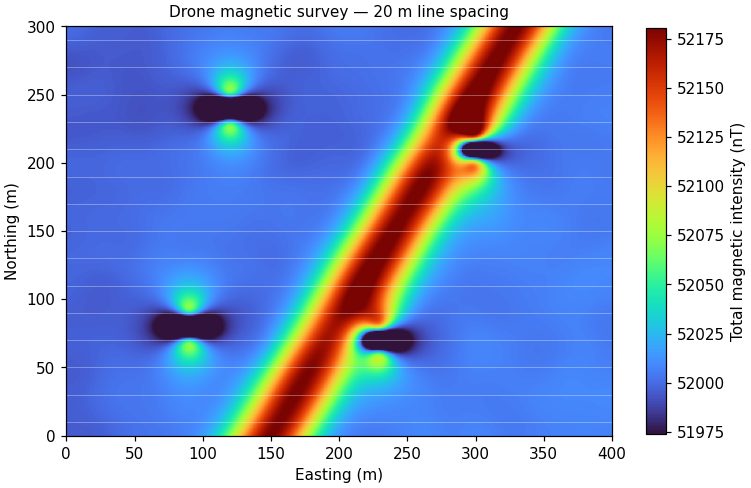
A lightweight magnetometer is flown beneath or ahead of a multirotor drone on pre-programmed lines. The instrument records the Earth's total magnetic field many times per second, and the processed grid shows where buried steel, magnetic rock units, faults and dykes disturb that field.

Terrain-following flight keeps the sensor at a steady height above ground. Data are corrected for diurnal variation using a base station, levelled between lines, and gridded. Derivative and reduced-to-pole products sharpen edges and place anomalies over their sources.

Low-altitude drones now carry frequency-domain EM sensors and air-launched ground penetrating radar. These systems map near-surface conductivity and layering over areas that are wet, soft, contaminated or otherwise hard to reach on foot.

The drone flies a few metres above ground at walking speed. EM coils measure the secondary field induced in conductive ground; radar antennas record reflections from interfaces. Both are positioned with RTK GNSS so results tie directly to site coordinates.

Every geophysical survey is easier to interpret on an accurate base map. We collect LiDAR point clouds and photogrammetric imagery by drone to produce bare-earth elevation models, contours and high-resolution orthomosaics.

LiDAR pulses pass through gaps in vegetation to reach the ground; photogrammetry reconstructs surfaces from overlapping photographs. Ground control and RTK positioning tie both to survey-grade coordinates.

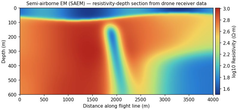
Semi-airborne electromagnetics pairs a grounded transmitter with a drone-borne receiver. A long cable laid on the ground drives a controlled, multi-frequency current into the earth, and a drone flies a magnetic-field sensor over the area to record the response. The result maps electrical resistivity to depths of several hundred metres, far deeper than other drone EM systems, without walking every line.

A grounded electric dipole, typically one to a few kilometres long, transmits a square-wave current at a set of frequencies. The drone tows a three-component induction-coil or fluxgate magnetometer on lines across and around the transmitter. Frequency-domain transfer functions are computed between the transmitted current and the received magnetic field, then inverted in 1D, 2D or 3D to resistivity-depth sections and volumes. One transmitter setup covers several square kilometres before it is moved.

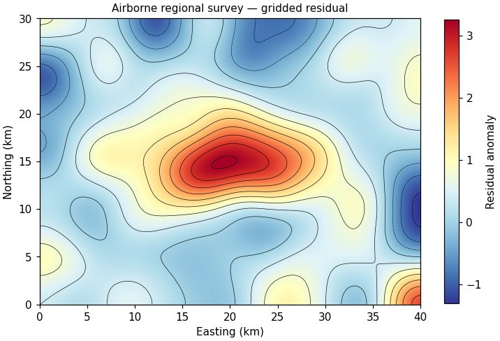
For areas measured in tens to thousands of square kilometres, helicopter and fixed-wing systems collect magnetics, time-domain EM, radiometrics and gravity. We design these programs, manage contractors, QC the data in the field and deliver the interpretation.

Survey aircraft fly parallel lines with tie lines for levelling. We specify line spacing, flight height and system to match the geological question, then check data daily against contract specifications before accepting it.

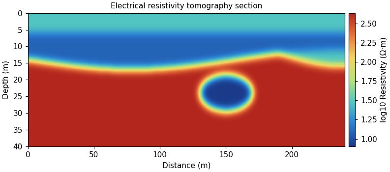
Electrical resistivity tomography (ERT) passes current through the ground between electrode pairs and measures the resulting voltage on many others. Inversion turns thousands of readings into a cross-section or volume of subsurface resistivity.

Clay, saline water and some ore minerals conduct; dry sand, gravel, fresh bedrock and voids resist. Mapping these contrasts outlines aquifers, contamination, fracture zones, bedrock depth and cavities.

Induced polarization (IP) is collected alongside resistivity and measures how the ground stores electrical charge. Disseminated sulfides, graphite and some clays hold charge and show up as chargeable zones.

After the transmitter current switches off, the voltage decays rather than dropping instantly. The size and shape of that decay (chargeability) is inverted with resistivity to map mineralized and altered ground.

Frequency-domain electromagnetic (FDEM) instruments use a transmitter coil to induce currents in the ground and a receiver coil to measure the response. No ground contact is needed, so large areas can be mapped quickly on foot, by vehicle or by drone.

The quadrature component maps apparent conductivity; the in-phase component is highly sensitive to metal. Multi-coil and multi-frequency instruments give several depths at once.

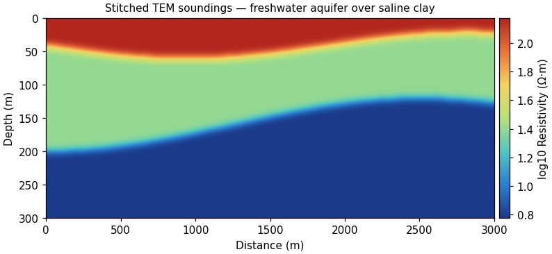
Time-domain EM (TEM) switches off a current in a large loop and records how induced currents diffuse into the ground. Early times see shallow layers and late times see deep ones, so each sounding gives a resistivity-depth profile.

Soundings are inverted into layered models and stitched into sections or 3D volumes. TEM sees through resistive cover to deep conductive targets and maps fresh/saline interfaces well.

Ground magnetometer surveys map the same magnetic field as drones but at the highest possible resolution, with the sensor carried or towed close to the ground.

Gradiometer configurations cancel regional field changes and highlight shallow objects. Walking surveys cover tight grids around structures where flying is not practical.

Gravity surveys measure tiny variations in the Earth's gravitational pull caused by density differences below ground. They map basin depth, faults, dense ore bodies and, at microgravity scale, voids and cavities.

Each station is precisely leveled and positioned. Readings are corrected for drift, tides, elevation and terrain (which is why accurate drone-derived elevation models matter) to produce Bouguer and residual anomaly maps.

Ground penetrating radar (GPR) transmits short radio pulses into the ground and records reflections from buried objects and layer boundaries. It gives the highest resolution of any surface method in the upper few metres.

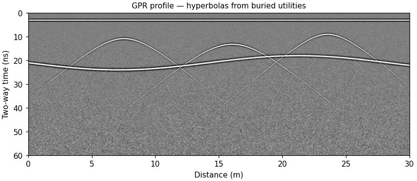
Antenna frequency sets the trade-off: high frequencies resolve rebar in concrete, low frequencies see deeper into soils. Hyperbolic reflections mark pipes and point targets; continuous reflectors mark layers and bedrock.

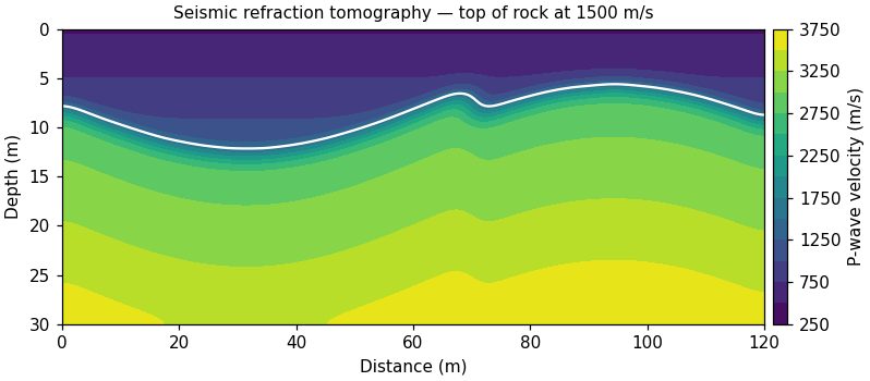
Seismic methods time sound waves from a hammer, weight drop or other source as they travel through the ground. Refraction tomography maps velocity and rippability; reflection images layer geometry at greater depth.

Geophones along a line record first arrivals. Velocity increases from soil to weathered to fresh rock, so the velocity model shows depth to bedrock and weak zones.

Multichannel analysis of surface waves (MASW) and passive methods such as HVSR measure shear-wave velocity, which is tied directly to soil stiffness and seismic site class.

Surface-wave dispersion is extracted from recorded data and inverted for shear-wave velocity with depth. Passive recordings use ambient noise and work in urban settings.

Borehole logging lowers probes down wells to measure natural gamma, resistivity, conductivity, temperature, fluid flow and acoustic or optical images of the borehole wall.

Logs tie surface geophysics to real geology, identify productive zones, locate fractures and verify well construction.

Towed resistivity streamers, boat-mounted GPR, magnetometers and bathymetric sonar extend our methods onto ponds, reservoirs and rivers.

Instruments are mounted on small boats or remotely operated vessels with GNSS positioning. Results combine water depth, sediment thickness and sub-bottom geology.